Deep Learning in Natural Language Processing
Quick overview of Deep Learning in NLP.
- Deep Learning in Natural Language Processing
Deep Learning in Natural Language Processing
I read many papers about Deep Learning (DL) in Natural Language Processing (NLP) in the starting months of my PhD. This blog is a summary of that reading, where I try to sequentially discuss the development of DL methods applied to various NLP tasks.
A little heads-up about the blog. This blog is not an in-depth analysis of DL methods applied to NLP tasks, instead, I have tried to provide a quick overview of the main development of DL methods for NLP. The goal of this post is to provide the reader with a direction for starting with DL in NLP. I’ll try to showcase the field’s evolution in a previous couple of years. Hopefully, by the end of this blog, if you are a newcomer to the field, you’ll at least have the understanding of technical terms of DL in NLP.
So, without further ado, let’s start.
Artificial Intelligence - Looking Back
First, a quick recap of the developments in Artificial Intelligence (AI) research. In the early days of AI, before the 90s, experts used to design task specific rules for different real-world problems. However, they would often fail when unseen or unexpected data/situation arrived.
In the last 20 years, around the late 90s or so, statistical approaches to these problems started gaining traction. Now, instead of writing rules, human effort was involved in extracting different features that would tell a mathematical model to learn the relation between input and output space. Statistical models are capable of learning the rules themselves, by looking at the labelled examples. These approaches can be considered as the early days of machine learning. However, they still require domain expertise to engineer domain specific features.
Around 2010, when a huge amount of data and powerful computers started coming out, a subset of machine learning, called deep learning, using neural networks became a model of choice for learning from data. These models are capable of learning the multi-level hierarchy of features and thus do not require any explicit need for feature engineering. Human energy is now focused on determining the most suitable architecture and training setting for each task.
From next sections, I’ll talk about NLP.
Word Embeddings
The first thing to start should be the representation of textual data in numerical format. Word Embeddings are used to represent words in a multi-dimensional vector form. A word wi in vocabulary V is represented in the form of a vector of n dimensions. These vectors are generated by unsupervised training on a large corpus of words to gain the semantic similarities between the words. Algorithms like word2vec [1] and GloVe [2] are used to train these word embeddings. These word embeddings are generally pre-trained and made publicly available to be directly used in the deep learning models.
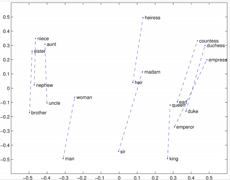
These distributed representations of words give a certain amount of semantic understanding of the words in a high dimensional vector space. For example, the distance between words king and queen will be similar to the distance between boy and girl. In this contrast, the below equation fits perfectly.
These representations have a drawback that they fail to take the context of a word into account. For example, the word ‘Scotland’ will have a different meaning in the sentence ‘Scotland is one of the best places to live on earth’ than in the sentence ‘Royal Bank of Scotland is one of the top banking firms in the UK’. The GloVe or word2vec word embeddings will fail to differentiate the two meanings of Scotland and will assign the same vector in both the cases. These drawbacks are tackled by a new concept of contextual word embeddings discussed in a section below.
- Other Resources
Sequence Learning
Most NLP tasks require sequential output instead of a single output label, unlike classification or regression, for example, Machine Translation, Question-Answering, or Named-Entity Recognition. These systems take a sequence of input and process it to produce yet another sequence for output. The goal is to take a sequence x1, x2, …, xn as input and map it to another sequence y1, y2, …, ym as output.
Vanilla seq2seq Model
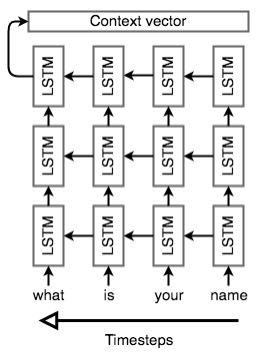
The architecture used to deal with this kind of problems is known as Sequence-to-Sequence model or in common terms, seq2seq model. It is a combination of encoders and decoders which works in a sequential manner, where, an encoder is a neural network that generates a context vector from the input sequence, and decoder, another neural network taking context vector as input, generates the output sequence.
The encoder takes an input X and maps it to fixed-size context vector Z using the formula given below:
where σ is an activation function. A decoder then maps the context vector Z to a new form of input X’ as shown in the equation below:
where σ’ is another activation function. The loss is calculated as the squared error between original and reconstructed input as shown in equation below:
An illustrated diagram of seq2seq model performing machine translation is shown in the figure below:
seq2seq with Attention
A problem with general encoder-decoder seq2seq model is that they give equal importance to all parts of the input sequence. Also, the input sequence is compressed into a single context vector which creates the bottleneck problem, where a piece of long information is tried to be compressed into one small representation.
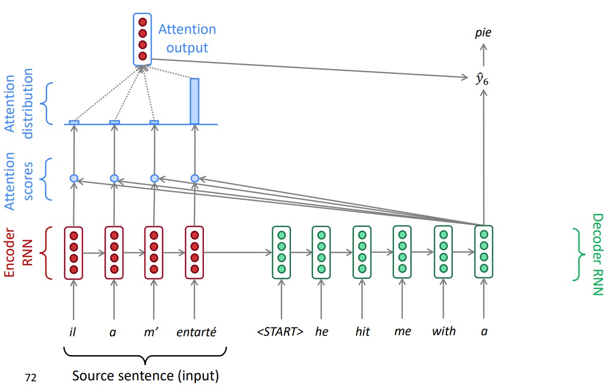
A solution to this problem was proposed in the work [3] introducing a new mechanism called Attention. Attention aligns the output at each decoding step to the whole input sequence in order to learn the most important part of the input aligning with the current step output.
Let’s say we have calculated the encoding hidden states h1, h2, …, hn for the input sequence x1, x2, …, xn during the calculation of context vector Z. For a decoder hidden state st on timestep t, we get attention score et as follows:
We take the softmax of these scores to get the attention distribution at timestep t.
The attention output at is then calculated as the weighted sum of encoder hidden state using ∝t:
Finally, we concatenate the attention output at with decoder hidden state st and proceed to calculate the negative log loss same as the non-attention decoder model.
An attentive machine translation model is shown in the figure below:
-
Other Resources
- Have a look at this lecture from CS224n.
- Read the seq2seq paper.
- Read this attention paper.
Learning Methods
Now let’s talk about the learning algorithms that are capable of learning the mapping between input and output representations. Here, we’ll take a look at some of the backbone neural networks (DL architectures) used in various NLP tasks.
Recurrent Neural Networks
Text is a sequential form of data. To process text and extract information from it, we need a model capable of processing the sequential data. Recurrent Neural Networks (RNNs) [4] are the most elementary deep learning architectures that are able to learn from sequential data. RNNs are wide in nature as they unroll through time. These networks will have a ‘memory’ component which can store the information about the previous state. They share the same set of weights throughout the layers, however, will receive a new input at every layer or time-step.
The output to every time-step is dependent on the input taken at the current time-step ti as well as the information gained from previous time-step ti-1. Specifically, an RNN will maintain a hidden state ht at every step which is referred as the memory of network. An illustrated diagram of unrolled RNN is shown in figure below
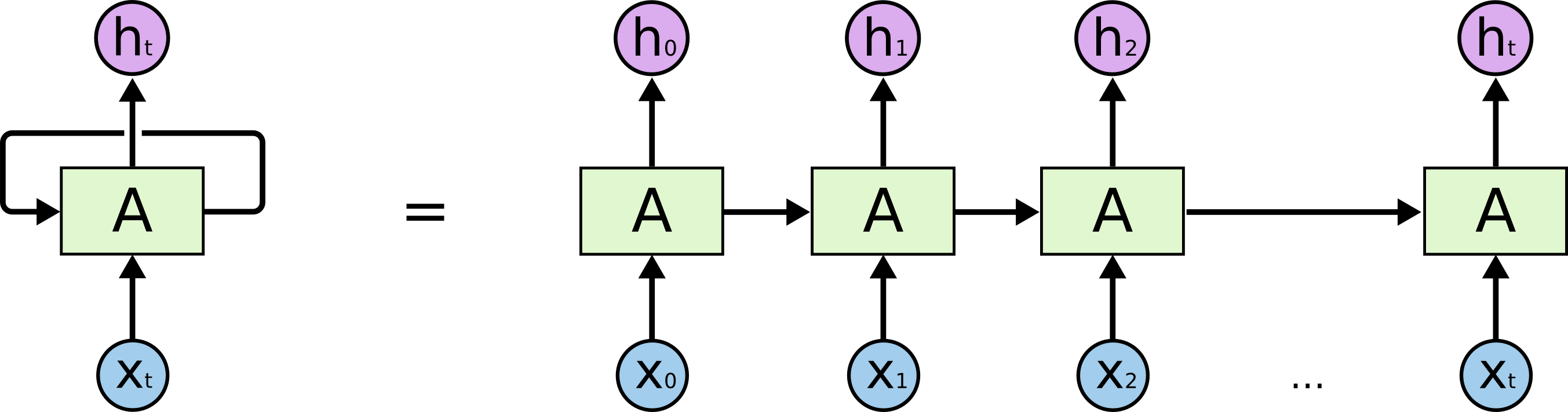
The operations performed in RNN at every time step is given in the equations below:
Here σy and σh are the activation functions. Wh is the weight matrix to apply transformation on previous hidden state ht-1, We is the weight matrix to apply transformation on the input xt received over time t. Combining these with the bias bh yields hidden state ht for time t. Applying activation on the ht with Wy gives the output yt for every time-step t.
-
Other Resources
- Have a look at this lecture from CS224n.
Long Short-Term Memory Networks
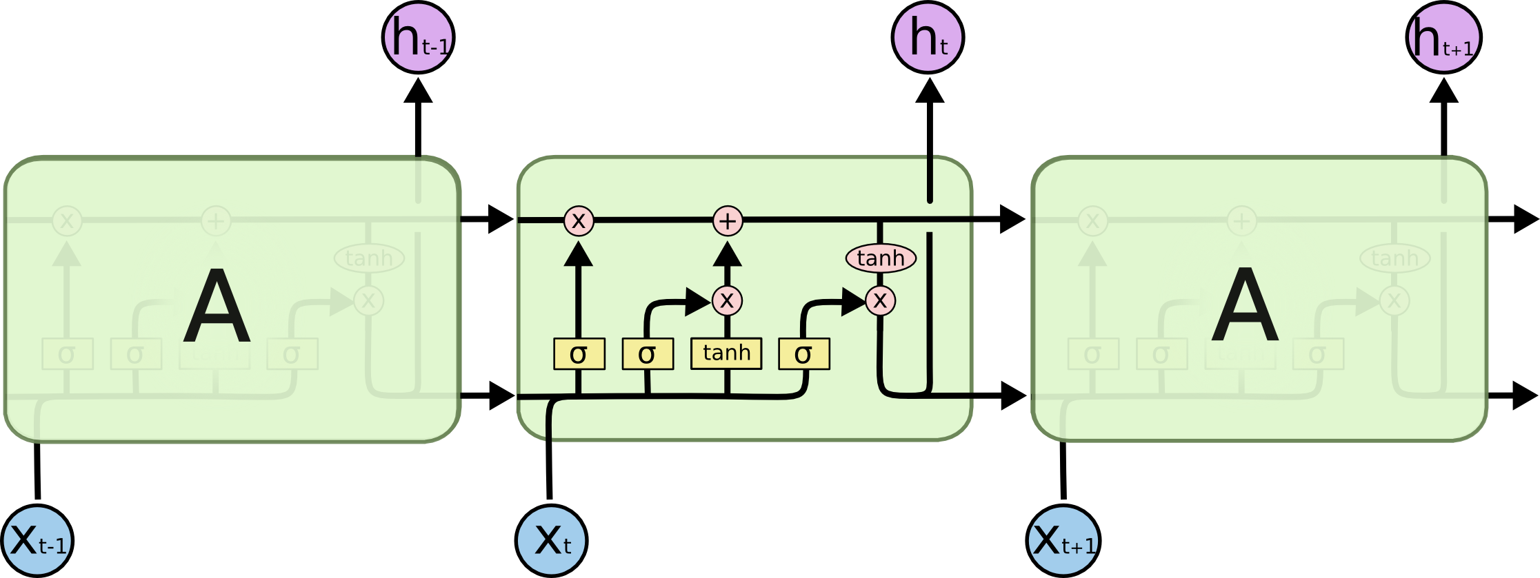
Although, in theory the RNNs are designed to handle the sequence input but in practice they lack in storing the long term dependencies because of the problem of exploding and vanishing gradients [5]. Long Short-Term Memory Networks [6] are the advanced version of RNNs with a slight modification of being capable of deciding what to ‘remember’ and what to forget from the input sequence with the help of a series of gates. LSTMs have a number of gates: an output gate ot; an input gate it; a forget gate ft - all of which are the functions of previous hidden state ht and current input xt. These gates interact with the previous cell state ct-1, the current input xt, and the current cell state ct and enable the model to selectively retain or information from the sequence. The full version of LSTM is given in the equation below.
where σg is the sigmoid activation function, σc and σh are the tanh activation function, and ○ is element-wise multiplication, also known as Hadamard product. An illustrated diagram of LSTM is shown below:
LSTM layers can be stacked on each other to form multi-layer LSTM architecture. One of the most popular LSTM architecture is Bidirectional LSTM (BiLSTM), where two separate LSTMs are used to capture the sequential information in both forward and backwards directions. Gated Recurrent Units (GRUs) [7] are another advanced version of RNN which are common for handling the vanishing gradient problem, but I am not discussing them here as they are almost similar to LSTM except with no cell-state.
-
Other Resources
- Go through this amazing blog from Christopher Olah.
Convolutional Neural Networks
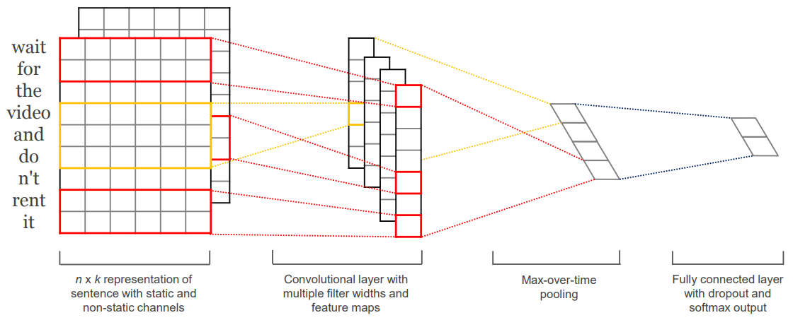
Convolutional Neural Networks (CNNs) [8] have established themselves as state-of-the-art in various computer vision tasks. For the last couple of years, CNNs have been the benchmark for almost every vision task. Inspired from the popularity of CNN in vision, Yoon Kim proposed a CNN architecture for sentence classification which outperformed then benchmarks on various text classification datasets [9].
A CNN takes an input sentence of n words, where each word is represented using a vector of dimension d. The input X1:n will be a 2D matrix of shape n × d, where xi ∈ ℝ d . Input X1:n can be represented as:
where ⊕ is the concatenation operator. On the input layer, convolution filter W ∈ ℝhd is applied over window of h words to generate a new feature. So, a feature ci is generated from the word window xi:i+h-1 with the following operation:
where W is the weight matrix for the connections, σ is the activation function and b ∈ ℝ is the bias. Now, this filter is applied to each possible window of words giving an feature map C ∈ ℝn-h+1.
The entries in feature map C are sharing the parameter W, where each ci ∈ C is a result of calculation on small segment of the input. Then a max-pooling operation is applied on these feature maps to capture the most important part.
This parameter sharing helps the model to incorporate an inductive bias into the model, helping to become learn the location invariant local features. There are k number of filters applied to the input with different window sizes which are then concatenated to form a vector K ∈ ℝk. Which is then fed to the next hidden layer or output layer.
An illustrated diagram of a CNN architecture for text classification is shown in the figure below:
-
Other Resources
- Have a look at the CNN for text classification paper.
- Also have a look at this lecture from CS224n.
Transformers
Most of the above models have recurrent behaviour, which can not be trained parallelly. This imposes a huge problem of time taken to train a model from scratch. In the work [10], authors proposed a new neural architecture called Transformers which uses a combination of self-attention and feed-forward network and doesn’t require any recurrent or convolutional elements. Also, the self-attention module lets the model capture the long term dependencies in a sentence without having any effect of the sentence length.
This new model was a huge success gaining better performance on various sequential learning tasks. To name one, it improved the machine translation performance by 10 BLEU on WMT EN-FR and WMT EN-DE datasets. It also reduced the training time by large margin benefiting from the non-recurrent behaviour.
The success of transformer architecture paved the way for the development of new models to solve the sequential tasks. It helped NLP researchers to utilize its non-recurrent nature in transfer learning where the transformer is used for general pre-training of a language model (LM). Then the LM fine-tuned on domain-specific dataset for downstream tasks. An encoder-decoder model using Transformer architecture is shown in the figure below:
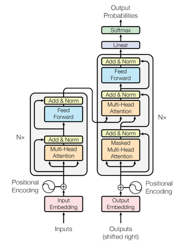
I cannot provide an in-depth overview of the Transformer but you can refer to resources below for a better understanding.
-
Other Resources
- Go through the main paper “Attention is all you need”.
- Take a look at this amazing blog.
- Must read - Jay Alammar’s blog on Transformers.
Language Models
Another important concept we should be aware of in NLP is Language Models (LM), because transfer learning in NLP is applied using different versions of LMs only. A language model is a type of system that predicts the probability of possible next words for a given sequence of words as the input.
In general terms, for a given sequence of input (x1, x2, …, xt) the probability distribution of next term (xt+1) is computed from a vocabulary V of k words (V = (w1, w1, …, wk)) as given below:
Earlier the language models were based on statistical approaches where they used to take a window of n words as a context from the sentence to predict the next word. This approach is also known as n-gram Language Model. It takes a simple approach of calculating the conditional probability of next word in the sentence given the window of n words as a context. These n-gram probabilities are calculated from counting them in some large corpus of text.
or in simpler terms:
This statistical approach has mainly two problems. First, sparsity - consider the above equation, what if w1, w2, w3 never occurred together, the probability of w3 will be 0. Second, storage - as we increase the value of n, the count of all n-grams we see in the corpus increases as well and so does the need of memory to store them.
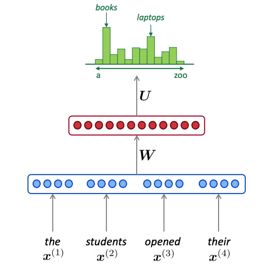
The neural language models using RNNs and Transformers are capable of modelling all the words in a sentence without needing a window to predict the next word at each timestep. You can think of a simple RNN for neural LM, where the RNN takes input tokens one at a time and by processing them generates the hidden state of each timestep. At the final time step, the output of that RNN block will be taken as the softmax against the whole vocabulary, and the word with the highest probability will be the prediction of LM as next word in the sequence.
-
Other Resources
- For a better and deeper understanding please refer to this lecture from CS224n.
Transfer Learning
NLP cracked transfer learning by applying a simple rule: first, learn the general nuances of text (grammar-rules or fill in the blanks) from a huge corpus of text using a language model; and then transfer that learning by fine-tuning the language model on a task-specific dataset. In the following sections, we’ll discuss some of the advancements in using different versions of LMs for transfer learning.
Embeddings Learned from Language Models
As discussed in the above section, the word embeddings generated by algorithms like word2vec and GloVe lack the contextual awareness and fail to differentiate a word with different senses. A new version of words embeddings, known as, contextual word embeddings are capable of differentiating a word’s sense based on its context. These new models use a Language Model (LM) to generate the contextualised representation of words in a sentence. These modified embeddings generated from the LMs can be used as the input to another neural network for some downstream tasks.
ELMo [11] is one such embedding algorithm that uses a bidirectional language model to capture the context of a word in a sentence from both sides (left to right and vice-versa). ELMo uses a character-level CNN to convert raw text into a word vector which is then fed into a bidirectional language model. The output of this BiLM is then sent to the next layer of BiLM to form a set of intermediate word vectors. The final output of ELMo is the weighted sum of raw vectors and the intermediate vectors formed from two layers of the BiLMs. The two language models used here are based on LSTM architectures. An illustration of ELMo is shown in the figure below:
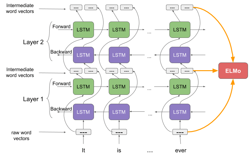
ELMo achieved 9% error reduction on the SQuAD (question-answering) dataset compared to then SOTA, 16% on Ontonotes SRL dataset, 10% on Ontonotes coreference dataset and 4% on CoNLL 2003 dataset. The fact that these embeddings are contextual and have the knowledge of word senses, helps ELMo and other future models such as BERT and GPT perform so much better.
-
Other Resources
- Before ELMo, CoVe proposed a similar idea. Have a look at the paper, if you fancy reading.
- Read the ELMo Paper.
- Recommended notes for a quick read.
- Have a look at this lecture from CS224u.
- Also, go through this amazing blog on Analytics Vidhya.
Universal Language Model Fine-Tuning
Universal Language Model Fine-Tuning (ULMFiT) [12] can be considered as one of the pioneers of applying transfer learning on an NLP task (text classification). It does so in three main steps: first, training a general domain-independent language model on a large corpus of text; second, fine-tune the language model on task-specific target dataset; and third, again fine-tuning the fine-tuned language model as a classifier by adding a softmax activation on top with target dataset. An illustration of the three steps of ULMFiT is shown in the figure below:
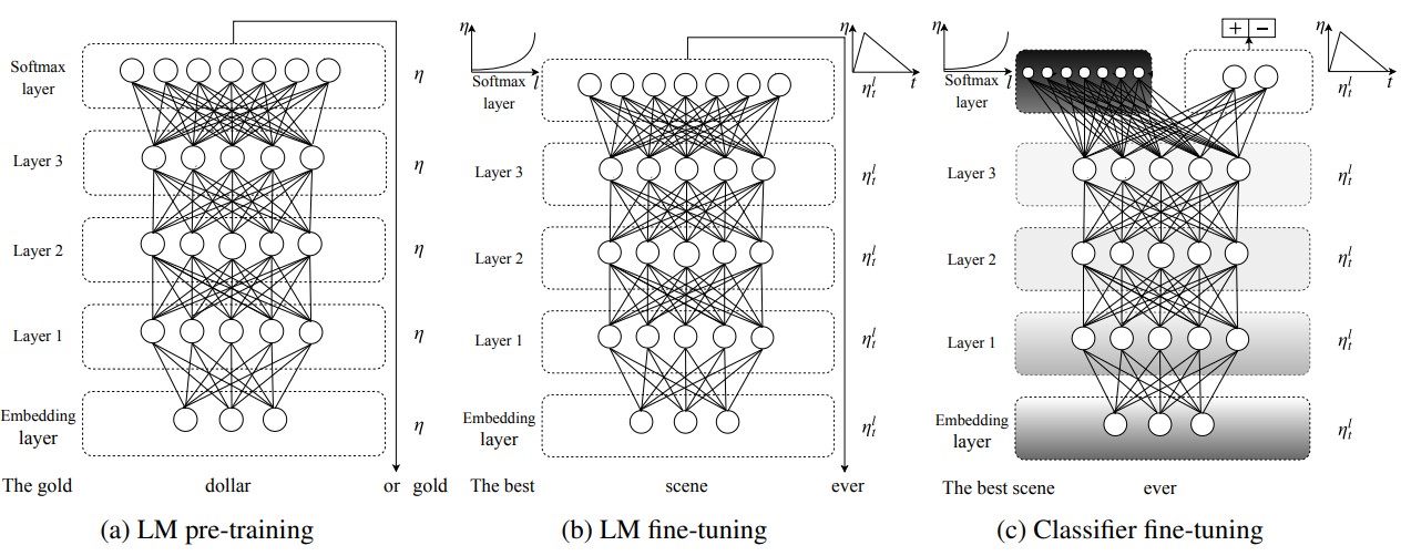
ULMFiT achieved better results for text classification on six different datasets ranging from topic classification to sentiment analysis. The fine-tuning approach employed by ULMFiT is also very interesting, where different learning rates are applied to different layers of the network. I would recommend reading the paper to get a better understanding of the updated version of backpropagation through time algorithm.
-
Other Resources
- Definitely read the ULMFiT Paper.
- Have a look at this amazing blog.
Generative Pre-Training
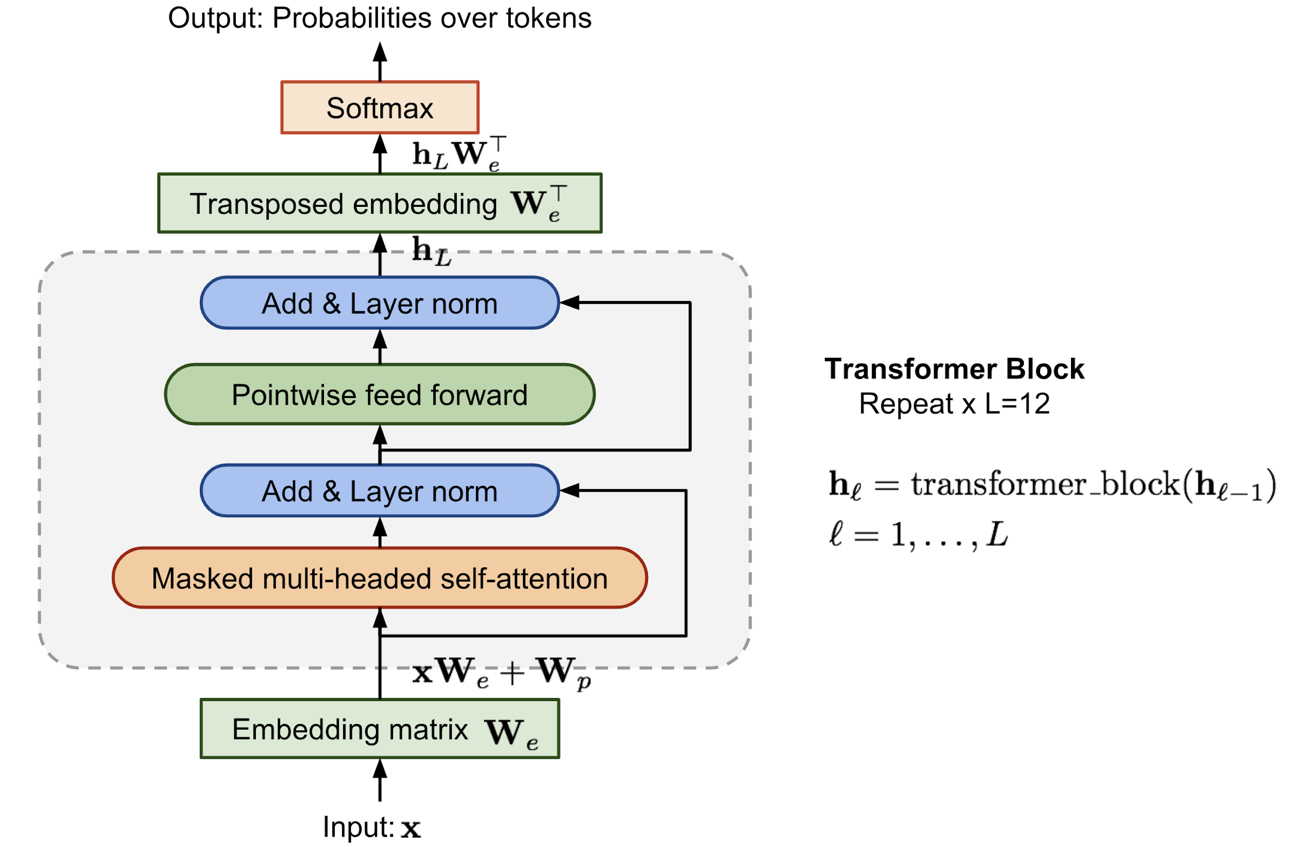
One of the earliest works in using Transformers for pre-training of language model and applying transfer learning was presented in Generative Pre-Training (GPT) [13]. Following the idea from ELMo, authors proposed a language model using transformer decoder trained on a large corpus of text. The main difference of GPT from ELMo is that ELMo uses two independent LSTM language models to capture the forwards and backward context whereas, in case of GPT, it uses a uni-directional multi-layer transformer language model capable of capturing context due to its attentive nature.
ELMo takes a feature-based approach of generating feature vectors (or contextual representations of the sentences) for different tasks, whereas GPT takes a fine-tuning based approach where the same language model trained on huge corpus is fine-tuned on task-specific data for downstream tasks. An illustration of a GPT model used for pre-training is shown in the figure below:
-
Other Resources
- Read the GPT Paper.
- The updated version GPT-2 Paper.
- A blog post similar to this one.
Bidirectional Encoder Representation from Transformers
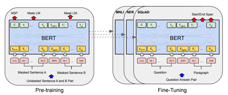
Bidirectional Encoder Representation from Transformers (BERT) [14] is another example of the success of transfer learning in NLP. BERT is a bidirectional transformer language model trained on a large text corpus that can be fine-tuned on any domain-specific dataset for the downstream tasks such as text classification, or named entity recognition. BERT mainly differs from other models like GPT and ELMo because of the pre-training tasks used during the unsupervised training of language model. Its pre-training is based on two tasks: first, Masked Language Model (MLM); and second, prediction of next sentence from the corpora.
For the first task of Masked Language Model, let’s say we have a sentence ‘Boris Johnson is the Prime Minister of UK’. So instead of training for prediction of next word in the sentence as a general Language Model, BERT pre-training replaces 15% of the words with a [MASK] token and learns to predict the correct word at the position of [MASK] token. In the second task of Next Sentence Prediction, the model is trained to learn the relationship between sentences where, for a given sentence pair A & B, the model is asked to predict if the sentence B is the next sentence that comes after A.
BERT improved the fine-tuning based approach of GPT by using a bidirectional transformer and learning both left & right context at the same time. This gave a huge improvement over GPT’s unidirectional approach especially for token-level tasks like Question Answering, where the answer depends on both left and right contexts. An illustrated diagram of BERT pre-training and fine-tuning is shown in the figure below:
A visual comparison between BERT, GPT and ELMo architectures presented in the paper is shown below:
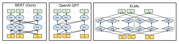
We can see, BERT uses the bi-directional transformer for processing the sequence, while GPT uses a uni-directional transformer. On the other hand, ELMo uses bi-directional LSTM to capture the bi-directional context while processing the input.
-
Other Resources
- Read the BERT Paper.
- Have a look at this amazing blog by Jay Alammar).
Further Steps
If you have made this far, then why not have some awesome resources for your further exploration.
- I would recommend looking at these amazing repositories:
- NLP-Progress: An open-source repo that tracks the SOTA in several NLP tasks in multiple languages.
- Awesome NLP: Another open-source repo providing a single place for many NLP resources.
- If you would like to study from some online courses, here are my top recommendations:
- fast.ai Course: A Code-First Introduction to NLP
- Stanford’s CS224n: Natural Language Processing with Deep Learning
- Stanford’s CS224U: Natural Language Understanding
Acknowledgement
-
The blog’s idea is highly inspired by Sebestian Ruder’s PhD thesis. Especially the background chapter, where a quick overview of deep learning is provided before proceeding to the contributions of the thesis.
-
I would like to thank Dr Muneendra Ojha and Krutika Bapat for reviewing the blog.
-
I took the help of numerous online resources to get a better understanding of this field. Some are listed here if I have missed any blog/resource - sincere apologies for that. Please comment here or write an email, I’ll properly acknowledge them.
References
[1] Mikolov, T., Sutskever, I., Chen, K., Corrado, G. S. & Dean, J. (2013), Distributed representations of words and phrases and their compositionality,in‘Advances in neural information processing systems’, pp.3111–3119.
[2] Pennington,J., Socher,R. & Manning,C. (2014), Glove: Global vectors for word representation, in ‘Proceed-ings of the 2014 conference on empirical methods in natural language processing (EMNLP)’, pp. 1532–1543.
[3] Bahdanau, D., Cho, K. & Bengio, Y. (2014), ‘Neural machine translation by jointly learning to align and translate’,arXiv preprint arXiv:1409.0473.
[4] Elman, J. L. (1990), ‘Finding structure in time’,Cognitive science14(2), 179–211.Graves, A., Jaitly, N. & Mohamed, A.-r. (2013), Hybrid speech recognition with deep bidirectional lstm, in ‘2013 IEEE workshop on automatic speech recognition and understanding’, IEEE, pp. 273–278.
[5] Bengio, Y., Simard, P., Frasconi, P. et al. (1994), ‘Learning long-term dependencies with gradient descent is difficult’, IEEE transactions on neural networks.
[6] Hochreiter, S. & Schmidhuber, J. (1997), ‘Long short-term memory’, Neural computation 9(8), 1735–1780.
[7] Cho, Kyunghyun, et al. “Learning phrase representations using RNN encoder-decoder for statistical machine translation.” arXiv preprint arXiv:1406.1078 (2014).
[8] LeCun, Y., Bottou, L., Bengio, Y., Haffner, P. et al. (1998), ‘Gradient-based learning applied to document recognition’,Proceedings of the IEEE86(11), 2278–2324.
[9] Kim, Yoon. “Convolutional Neural Networks for Sentence Classification.” Proceedings of the 2014 Conference on Empirical Methods in Natural Language Processing (EMNLP). 2014.
[10] Vaswani, A., Shazeer, N., Parmar, N., Uszkoreit, J., Jones, L., Gomez, A. N., Kaiser, Ł. & Polosukhin, I.(2017),Attention is all you need, in‘Advances in neural information processing systems’, pp.5998–6008
[11] Peters, M. E., Neumann, M., Iyyer, M., Gardner, M., Clark, C., Lee, K. & Zettlemoyer, L. (2018), ‘Deep contextualized word representations’,arXiv preprint arXiv:1802.05365.
[12] Howard, J.&Ruder, S.(2018), ‘Universal language model fine-tuning for text classification’, arXiv preprintarXiv:1801.06146.
[13] Radford, A., Narasimhan, K., Salimans, T. & Sutskever, I. (2018), ‘Improving language un-derstanding by generative pre-training’.
[14] Devlin, J., Chang, M.-W., Lee, K. & Toutanova, K. (2018), ‘Bert: Pre-training of deep bidirectional transformers for language understanding’, arXiv preprint arXiv:1810.04805.